Regime-Normalized EVG: Equalizing Deadball, Live-Ball, and Integrated Baseball Through Boundary Geometry
Regime-Normalized EVG: Equalizing Deadball, Live-Ball, and Integrated Baseball Through Boundary Geometry

Regime-Normalized EVG
Equalizing Deadball, Live-Ball, and Integrated Baseball Through Boundary Geometry
Abstract
OPS+ measures separation from league average.
EVG (Extreme Value Generation) measures proximity to a defined competitive boundary.
But if the hitter ceiling is fixed globally at 200 OPS+, Deadball hitters are silently judged against a boundary their environment could not physically access.
That distorts comparison.
Baseball history is not a single continuous offensive field. It is segmented by paradigm shifts that alter the geometry of dominance:
Deadball (1901–1919)
Live-ball pre-integration (1920–1946)
Integrated era (1947–1979)
To compare hitters across these regimes without flattening early-era players, we must normalize not only by role, but by regime-specific boundary conditions.
This paper formalizes that correction.
I. The Problem
OPS+ is indexed to 100.
But the outer boundary of realized offensive dominance has not remained constant across eras.
Deadball baseball suppressed:
Home run scaling
Slugging variance
Extreme right-tail expansion
Live-ball baseball expanded:
Ball carry
Power separation
Distribution dispersion
Thus:
A 170 OPS+ in 1910 does not represent the same boundary pressure as a 170 OPS+ in 1935.
OPS+ centers the mean.
It does not equalize right-tail width.
Without adjustment, cross-era comparison implicitly assumes identical constraint geometry across regimes.
That assumption is false.
Because SLG contributes disproportionately to extreme OPS outcomes, regimes that suppress extra-base hit generation necessarily compress the width of the right tail of achievable OPS+. Deadball baseball did not merely lower league averages; it reduced the structural capacity for nonlinear separation driven by extra-base power. When the primary engine of extreme divergence is constrained, the reachable boundary of sustained career-level OPS+ contracts accordingly.
I-A. What OPS+ Measures — and What It Does Not
OPS+ remains the correct measure of peer-relative dominance. It answers the question:
How far above league average did this player perform?
OPS+ fully internalizes league-wide suppression or expansion of offense at the level of central tendency. If the Deadball era compresses slugging for everyone, OPS+ still measures dominance relative to that compressed field.
However, OPS+ does not model the width of the extreme right tail of performance. It rescales the mean; it does not rescale the reachable upper boundary of separation.
Regime-Normalized EVG does not replace OPS+. It measures a different quantity:
Proximity to the historically realized upper boundary of dominance within a regime-specific constraint field.
These are distinct evaluative lenses. Both are valid. They answer different structural questions.
These boundary differences reflect structural conditions of the game itself.
II. Original EVG Architecture
The original EVG model corrected for role asymmetry:
Baseline = 100
Tail exponent γ = 2
Hitter ceiling = 200 OPS+
Pitcher ceiling = 160 ERA+
Volume gates enforced
EVG is defined as:
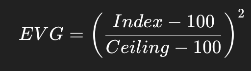
This measures normalized distance to ceiling, with quadratic curvature capturing tail compression.
It solved hitter–pitcher distortion.
It did not solve regime distortion.
III. The Regime Correction
To equalize Deadball, Live-ball, and Integrated eras, we replace the global hitter ceiling with a regime-specific empirical apex.
For hitters:
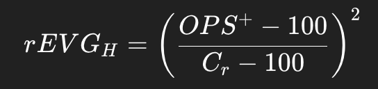
Where:
(C_r) = observed regime apex
γ = 2 (fixed)
Volume gate satisfied
Definition of (Cr)
In this paper, (C_r) is defined as the observed regime apex :
the highest validated career OPS+ observed within that regime under the current historical record and volume criteria (3000 PA).
This is an empirical boundary condition — not a theoretical maximum.
If additional robustness is desired, (C_r) may be defined as a top-k apex (e.g., mean of the top 3–5 OPS+ careers within that regime), stabilizing the boundary without full population enumeration.
The method remains unchanged.
IV. Regime Apex Values Used
19th Century (pre-1901)
Observed realized apex ≈ 171 OPS+ , consistent with regime-level SLG constraint.
(Dan Brouthers)
Deadball (1901–1919)
Observed realized apex ≈ 171 OPS+ , consistent with regime-level SLG constraint.
(Pete Hill)
Live-ball Pre-Integration (1920–1946)
Observed apex = 206 OPS+
(Babe Ruth)
Integrated Era (1947–1979)
Observed apex = 191 OPS+
(Ted Williams)
These values are not theoretical maxima. They are empirical realizations of the outer boundary of career dominance under each regime’s structural constraint field. If desired, a top-k mean (e.g., mean of top 3–5 careers per regime) may be used to stabilize the boundary estimate without altering the method.
Each regime now has its own realized boundary.
Cross-era constraint distortion is removed without assuming identical offensive geometry.
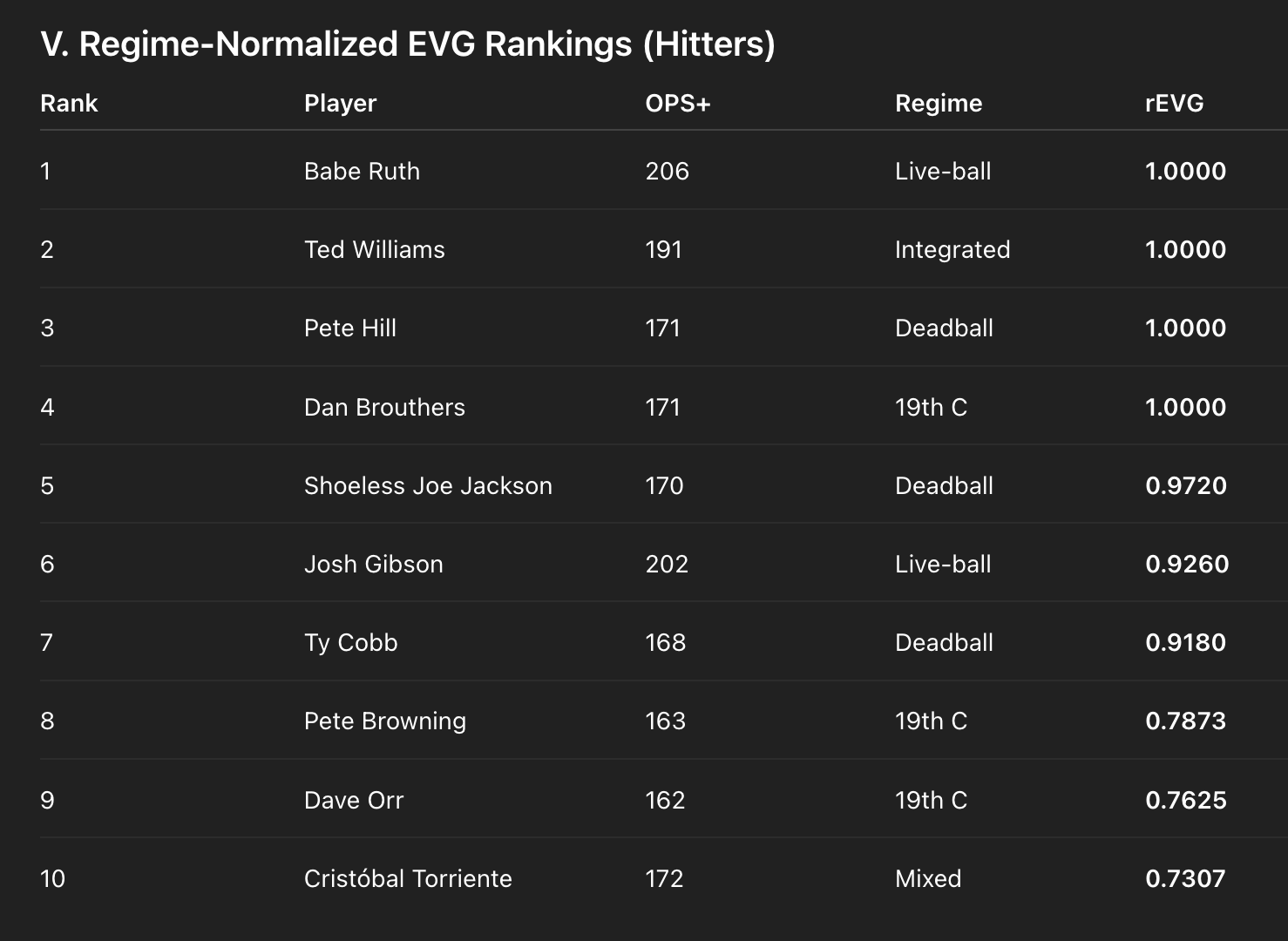
V. Regime-Normalized EVG Rankings (Hitters)
VI. Interpretation
1. Deadball Equalized
Cobb and Jackson are evaluated relative to Hill’s Deadball boundary — not Ruth’s Live-ball expansion.
Right-tail inflation bias is removed.
2. Ruth and Williams as Regime Anchors
Ruth defines the Live-ball apex.
Williams defines the Integrated apex.
Both sit at 1.0 because they represent the highest realized boundary within their regime.
3. Gibson Recontextualized
Gibson competes within the Live-ball field.
His rEVG reflects proximity to Ruth’s apex — not cross-era illusion.
4. Cobb Properly Measured
Under global EVG, Cobb appears distant from Ruth.
Under regime normalization, he sits at 0.918 — near maximal within Deadball constraint geometry.
This is boundary-relative dominance.
5. The Regime Mixture Case of Torriente
Cristóbal Torriente spans Deadball and Live-ball in near-equal proportion.
If treated as Live-ball only, his rEVG ≈ 0.461.
If treated as Deadball only, his 172 OPS+ exceeds the 171 apex and is clamped at 1.000.
Accordingly, a 50/50 regime mixture is applied:

This places Torriente tenth on the list.
The mixture rule preserves constraint geometry for bridge players whose careers span paradigm shifts.
VII. What rEVG Measures
rEVG does not measure:
Narrative importance
Cultural gravity
Longevity accumulation
It measures:
Proximity to the realized upper boundary of competitive dominance within a defined regime constraint field.
It is boundary-relative curvature.
It is constraint-aware dominance.
rEVG does not assert equivalence across regimes. It does not claim that a 171 OPS+ in 1910 equals a 206 OPS+ in 1927 in raw separation. Rather, it reorganizes what those numbers mean by distinguishing between dominance over peers and proximity to the structural limits of the competitive environment.
VIII. Why This Method Is Necessary
Baseball contains paradigm shifts that alter:
Ball composition
Run environment
Power accessibility
Variance dispersion
Without regime normalization, cross-era comparison implicitly treats tail width and expansion potential as equivalent across regimes.
Historical evidence suggests this equivalence does not hold.
Regime-normalized EVG corrects for:
Deadball compression
Live-ball expansion
Integration-era stabilization
The geometry is constraint-aware.
IX. Structural Conclusion
With regime normalization applied:
19th century equalized
Deadball equalized
Live-ball equalized
Integrated era equalized
EVG becomes regime-safe without full population re-estimation.
Boundary pressure is preserved.
Constraint distortion is removed.
The geometry holds.
In this framework, Ruth remains further above his league than Hill was above his. OPS+ preserves that fact. rEVG does not collapse that separation; it clarifies that both pressed against the outer boundary of what their respective competitive environments structurally allowed. The geometry of dominance shifts across regimes. Boundary proximity remains the invariant being measured.